The Model of Temporal Inertia
The Science Behind Targeted Seasonal Forecasts

The Model of Temporal Inertia: How Time Series Forecasting Operates
All science is predictive. The point of science is to be able to predict what an outcome will be. We accomplish this by applying the scientific method. We begin by observing a phenomenon and creating a hypothesis to describe what it is. When we’ve gathered enough evidence by testing the hypothesis, we can build a model that explains how the phenomenon occurs. When we understand how something happens, we can formulate a theory that explains why it happens. Once we have a valid theory of why something happens, and working model of how it happens, we can be confident of our ability to predict what will happen.
Since the introduction of the scientific method, we have developed sufficient laws, theories, and models to predict most physical, chemical, and biological phenomena. We have a comprehensive understanding of the dimension of form and the material world. However, we lack a framework to predict temporal phenomena.
Put another way, we have absolutely no idea how time series forecasting operates.
We have extensive evidence that it’s possible to predict what a future value will be. And the theory of probability explains why it’s possible to infer future outcomes based on the odds. But we don’t have a model that explains exactly how patterns in the past are able to predict future outcomes.
Not to put too fine a point on it, but the entire science of time series forecasting is based on the assumption that patterns in the past will continue in the future, and this is a problem. Assumptions are not scientific, and assumptions can’t be tested. If we don’t understand how time series forecasting works, we can’t improve it and move beyond the current limitations.
The current paradigm of time series forecasting faces three significant problems, each of which limits how confident we can feel about the forecast results.
First, even when combined with AI the forecast models require stationary time series data. The greater the variability and randomness of the historical data, the less confident we can feel about the forecast values. Second, even with AI, the forecast horizon is limited to a single period. We can have confidence in only the first forecasted value; the margin of error of each subsequent forecasted value increases exponentially. Third, unless seasonality is detected and used in the forecast model, the forecast consists of a single value. It’s possible only to forecast the trend ( what ) but not to forecast the variability ( when ).
The Model of Temporal Inertia solves these problems. It provides a valid, compelling, supported explanation of how time series forecasting works, and connects the what of the forecasts to the why of probability theory. It eliminates the need for stationary data, provides a robust alternative to the single-period forecast horizon, and produces forecasts that capture both trend and variability, even without seasonality.
The Model of Temporal Inertia
Newton’s First Law of Motion, the Law of Inertia, states that an object at rest remains at rest, and an object in motion remains in motion in constant speed and in a straight line unless acted on by an unbalanced force. This would seem to describe the behavior of time series forecasts where we assume that a pattern of behavior in time series data will continue, except we assume that the Law of Inertia exclusively applies to the dimension of form and not to the dimension of time. We assume this because of the limits of human perception, and specifically because of the limited ability of human beings to perceive the dimension of time.
We accept that the Law of Inertia governs everything about the position of an object in space, but this is not entirely accurate. The Law of Inertia determines the position of an object in space and time. The Law of Inertia already applies to the dimension of time, and therefore, it can function as the foundational theory to explain why time series forecasting works.
The Law of Inertia states that the velocity (speed and direction) of an object moving through space and time remains constant until acted on by an unbalanced force. The Model of Temporal Inertia proposes that the values of data organized in a time series will follow the same trend (speed and direction) until acted on by an unbalanced force.
To understand how time series forecasting works, we require a model. A model makes it possible to connect a hypothesis (the what of an observed event) to a theory (the why).
The velocity (speed and direction) of a moving object can be modeled as an x-t graph (Figure 2-1), where the y-axis represents the velocity, and the x-axis is time.

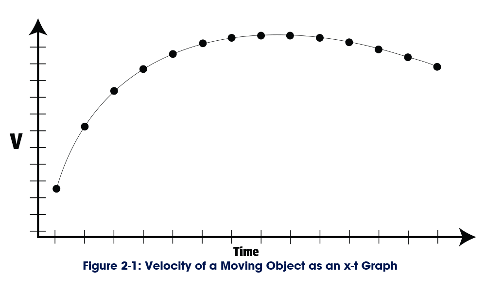
While the V in Figure 2-1 might correspond to the velocity of an object in motion, what it actually represents is “value.” The x-t graph that models the velocity of an object in motion is identical in every respect to a plot of time series data. This means that every mathematical formula that defines, explains, and predicts the values of the velocity of an object in motion also defines, explains, and predicts every value in a set of time series data.
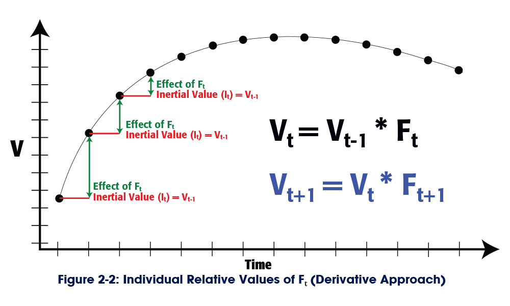
The velocity of an object in motion at a single point in time (Vt) is the product of the inertia of that object at that point in time (It) and the cumulative effect of the unbalanced forces acting on that object at that point in time (Ft). We can take this to mean that the value of an observed datum in a time series at a single point in time (Vt) is the product of the inertia of the time series (It) and the cumulative effect of the unbalanced forces (Ft) acting on the time series. We can express this as Vt = It * Ft.
When considering the movement of a physical object, each of these three factors can be observed and quantified independently at each point in time.
We can quantify the speed and direction (velocity) of the object through direct observation. The three main unbalanced forces that act on a physical object in motion are gravity, lift, and drag. As long as we know the physical properties of the object, we can calculate the effects of each of these forces at each moment in time. The inertia of the object depends on the mass of the object, which is constant, and the distance from the axis of rotation, which varies with motion. While it’s possible to calculate the precise inertia of an object, it’s extremely difficult.
Thanks to the Law of Inertia, we don't need to calculate the value of It.
The Law of Inertia states that the value will remain constant over time unless acted on by an unbalanced force. So the inertia of a point in time is equal to the value at the previous point in time. We can express this as It = Vt-1. This means that we can eliminate one factor from the equation and work with Vt = Vt-1 * Ft.
The formula to forecast the next value in the series is therefore Vt+1 = Vt * Ft+1.
In theory, we can continue with this approach to forecast additional values in the series, using the derivative approach illustrated in Figure 2-2. The problem with the derivative approach is that the margin of error of each subsequent forecast value increases exponentially.
The first forecast period always has the lowest possible error.
We can be entirely certain that the inertia of the forecast period is equal to the observed value of the previous period. We can’t know the value of Ft+1, so that’s the factor that introduces the error, Ft+1(E). We can express the forecast like this: Vt * Ft+1(E) = Vt+1(E).
The formula to forecast the next value in the series is Vt+1(E) * Ft+2(E) = Vt+2(E2). Because both factors include an error, the margin of error in the second forecast is the square of the margin of error in the first forecast. The error in the third forecast is the cube of the error in the first forecast: Vt+2(E2) * Ft+3(E) = Vt+3(E3). The expected error of each forecast period increases exponentially, and the confidence in each subsequent forecast value plummets accordingly.
If we take an integral approach to forecasting, we can address the problem of exponentially increasing errors.
If we take an integral approach to forecasting, we can address the problem of exponentially increasing errors. The relative value of Ft, which can be expressed as rFt, can be calculated relative to a common denominator, such as the mean value of the time series (MVts) (see Figure 2-3).
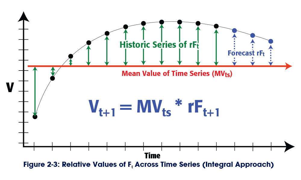
The MVts is a constant, rather than a variable, so it doesn’t introduce a new error into the forecast. The only variables that introduce the errors are the forecasted values of rFt. Each value of rFt has its own margin of error, but those errors are not necessarily dependent on each other and they don’t necessarily increase.
The formula to forecast the first value in the series is MVts * rFt+1(E1) = Vt+1(E1). The formula to forecast the second value in the series is MVts * rFt+2(E2) = Vt+2(E2). And the formula to forecast the third value in the series is MVts * rFt+3(E3) = Vt+3(E3).
This is possible only if each rFt value is forecast independently and is the product of a single-period forecast. We can’t do this with a single-timeline model, but we can do this if we consider the series of rFt values along the seasonal timeline.
Seasons of Time and the Seasonal Timeline
Human beings model time as a single dimension: a timeline. Your direct experience of time is limited to the present moment. The only correct answer to the question, “What time is it?” is “Now.” It’s always “now.”
You remember other nows that are not the now that you experience now, and you call these “then,” and you anticipate nows that you have yet to experience, and you call these “later.” The calendar and the clock provide objective references to organize the sequence of subjective “thens” and “laters,” but your actual, subjective, personal experience and perception of time is limited to the present moment, and the present moment orients you on the sequential timeline.
“Now” is a single point on the sequential timeline, but a point has no dimension and therefore can’t be measured. Each unit of measurement of time describes a segment of the sequential timeline that contains an infinite number of points. Each point in time has a corresponding value, which means that the value associated with a unit of time is the mean value of the infinite number of points contained within the segment.
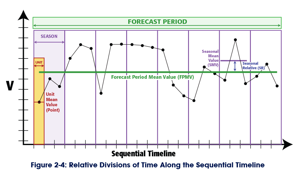
We require a minimum of three coordinates to orient ourselves along the sequential timeline: a period, a season, and a unit.
Each of these represents a segment of the sequential timeline, arranged in a hierarchy. A period is a sub-division of the sequential timeline itself; a season is a sub-division of a period; and a unit is a sub-division of a season. Each segment defines the boundaries of a mean value. The Seasonal Mean Value (SMV) is the mean of the Unit Mean Values within a season. The Forecast Period Mean Value (FPMV) is the mean of the Unit Mean Values within the forecast period. And the Seasonal Relative (SR), the relative effects of the unbalanced forces that we’ve been calling rFt, is the ratio of the SMV to the FPMV (see Figure 2-4).
Seasons allow us to orient units within the forecast period.
A season describes one or more of units (points) in time grouped together by a defining characteristic. The seasonal model establishes the defining characteristics that will be used to segment the larger population of time.
When we think of time, we think of the sequential timeline.
The sequential timeline is what is represented by the x-axis when we model time series data. The sequential timeline organizes contiguous events in a linear sequence moving from the past to the future. The seasonal model divides the sequential timeline into contiguous seasons. On the sequential timeline, Season 8 2025 follows Season 7 2025, which follows Season 6 2025.
The seasonal timeline organizes successive, non-contiguous instances of individual seasons within a seasonal model.
On the seasonal timeline, Season 8 2025 follows Season 8 2024, which follows Season 8 2023.
We’re most familiar with seasonal models that correspond with calendar- or clock-based units of measurement, such as a calendar month or the week of the year. However, the defining characteristics of a season are not limited to the units of the calendar or the clock, and seasons may not be comprised of contiguous and consecutive units (points).
Figure 2-5 divides the sequential timeline into eight seasons. Each season contains three Unit Mean Values. The SMV of each season is the mean of the three values in the season, and the SR is the ratio of the SMV to the FPMV. To forecast the SMV of Season 5 2025, we need only determine the forecasted Seasonal Relative (FSR) of Season 5 and multiply it by the FPMV.
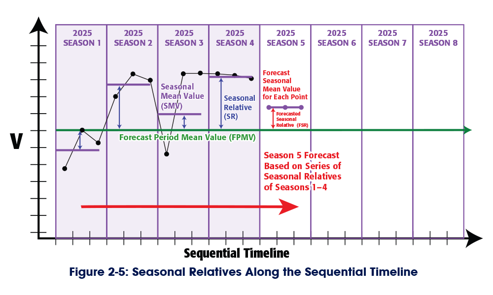
If we forecast the FSR along the sequential timeline, we're using a derivative approach.
The FSR of Season 5 2025 is dependent on the SR of Season 4 2025. We can be confident of this forecast because it has the smallest possible margin of error. However, we can’t expand the forecast horizon because the FSR of Season 6 would be dependent on the FSR of Season 5, which increases the error exponentially.
If we forecast the FSR along the seasonal timeline, we're using an integral approach.
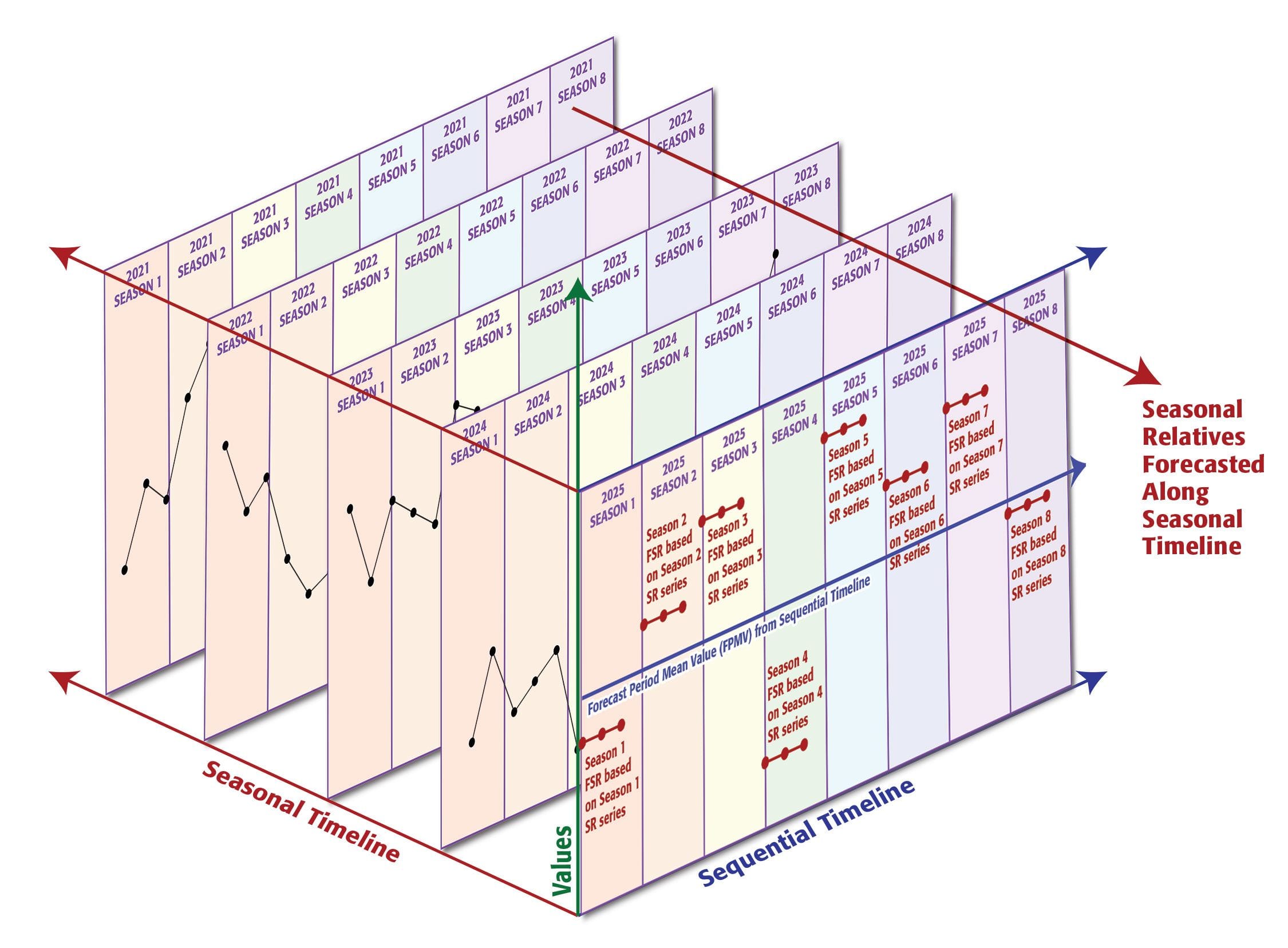
The FSR of Season 5 2025 is dependent on the SR of Season 5 of 2024. We can forecast the FSR of Season 6 2025 with the same level of confidence because the FSR of Season 6 2025 is dependent on the SR of Season 6 2024. To fully appreciate this, we need a three-axis graph that includes both the sequential timeline and the seasonal timeline (Figure 2-6).

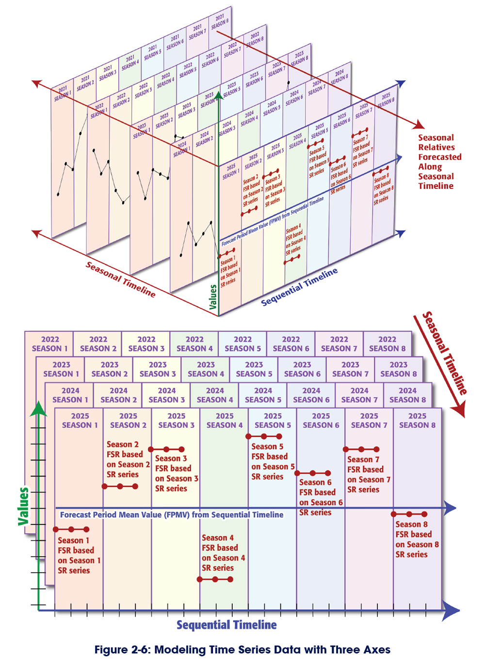
The forecast of each season along the sequential timeline is the product of two single-period forecast values from two different time series on two different timelines.
The single-period forecast for the sequential timeline is the FPMV. The FSR of each season is the product of its own single-period forecast along the seasonal timeline. Because each forecast value is independent, the errors do not increase exponentially and we can have a consistent level of confidence in the forecast for each season along the sequential timeline.
This forecast model captures both the trend (mean values within each season) and variability (different mean values between seasons).
Non-Stationary Data and the Model of Temporal Inertia
Classical forecast models perform best when forecasting with stationary data, where the values remain relatively constant and exhibit limited variability. When looking for patterns in the historical data, classical forecast models must filter out the noise — the so-called random component of the time series data. AI and machine learning models look for additional patterns in the noise in the hopes of producing a more accurate forecast value, but even so, the more random the time series data is, the less confident we can be in the results of classical forecast models.
The Model of Temporal Inertia explains the source of this problem and overcomes it.
Non-seasonal classical forecasts produce a single forecast value that extends across the entire forecast horizon. This unchanging trend is in fact, the Forecast Period Mean Value (FPMV). In other words, non-seasonal classical forecasts are forecasting the inertial trend, and ignoring the relative effects of the unbalanced forces.
To forecast the inertial trend, classical forecasts must isolate the effects of the unbalanced forces by transforming the data to make it stationary. When viewed through the Model of Temporal Inertia, the non-stationary components of time series data, including trends, cycles, seasonality, and the “random” noise, are the cumulative relative effects of unbalanced forces, which are modeled as seasonal relatives.
In the Model of Temporal Inertia, each forecast value is the product of the FPMV (the inertial trend) and the FSR. It’s a two-step process that requires two forecast values. Classical forecast models address only step one, the FPMV. The Model of Temporal Inertia addresses the FSR and completes the second step. It doesn’t require stationary data because it’s able to quantify the relative effects of the unbalanced forces and identify when those forces are expected to change (i.e., between seasons).
Conclusions
The Model of Temporal Inertia addresses each of the foundational problems that limit the confidence in classical time series forecasts. The Model of Temporal Inertia does not require stationary data and is able to generate forecasts with untransformed, raw data. Rather than isolating and discarding the random elements of data, the Model of Temporal Inertia captures those elements as seasonal relatives and forecasts when the effects of the unbalanced forces are expected to change.
The single-period forecast horizon is the consequence of forecasting on a single timeline.
We can be confident of only the first forecast value on a single timeline. The margin of error of each subsequent forecast value increases exponentially. The Model of Temporal Inertia expands the forecast horizon by forecasting multiple periods at once and assembling the series of single-period seasonal forecasts along the sequential timeline. Each seasonal forecast is the product of two single-period forecast values on two different timelines: the FPMV is forecast along the sequential timeline, and the FSR is forecast along the seasonal timeline. Because each seasonal forecast is independent, they maintain a consistently high level of confidence.
Additionally, because the forecast value of each season along the sequential timeline is independent, the forecast captures both trend (within each season) and variability (between seasons).