
Patterns in time exist, but we can’t perceive them directly. Science relies on observation. We can’t understand something if we can’t see it. Sometimes we need new tools to help us to see things that are invisible to the naked eye.
Before the invention of the microscope, the concept of a biological cell didn’t exist. Robert Hooke, a British scientist with an impressive resume of discoveries, coined the term “cell” after viewing a thin slice of cork under a microscope. Hook stated in 1665,
“…by the help of Microscopes, there is nothing so small as to escape our inquiry; hence there is a new visible World discovered to the understanding.”
The invention of the microscope made the entire science of microbiology possible, and has led to countless advancements in chemistry and physics.
Think of the Model of Temporal Inertia as a Microscope for Time.
When you view a drop of water through the lens of a microscope, you can see a world of single-cell organisms that are otherwise invisible. When you view time series data through the lens of the complex, irregular seasonal models that I’ve developed, you can see patterns and cycles that are otherwise invisible. Those patterns allow us to see further into the future with greater detail, precision, and confidence than possible with any existing tool. Each seasonal model is a lens in the Microscope for Time, revealing patterns of unbalanced force along the seasonal timeline.
Seasonal Models: Lenses in the Microscope for Time
The ways that we measure and divide time are based on repeated cycles or seasons. A season describes a number of units of time grouped together by defining characteristics. The seasonal model establishes the defining characteristics that will be used to segment the larger population of time. Some of the defining characteristics include calendar-based, contiguous, consecutive, and consistent.
A seasonal model is calendar-based if the seasons are defined as divisions of the calendar year (days, weeks, months, quarters). Every season occurs during every calendar year. If a seasonal model is not calendar-based, a calendar year may not include instances of every season.
A seasonal model is contiguous if the seasons consist of multiple contiguous data points (i.e., a contiguous group of days). A seasonal model is non-contiguous if a season consists of multiple non-contiguous data points (i.e., Mondays in January).
A seasonal model is consecutive if the seasons always follow a fixed order (i.e., the days of the week, the months of the year). A seasonal model is non-consecutive if the order of the seasons can vary.
A seasonal model is consistent if the duration of each season is fixed, unchanging, and equal. A seasonal model is inconsistent if the duration of a season can vary from instance to instance, or if the seasons are not at least approximately equal in duration.
When we think of seasons, we think of the calendar, and it’s hard to think of seasons that aren’t based on the calendar. We have five calendar-based seasonal models to choose from when working with daily aggregated data: Calendar Month, Week Year, Week Day, Month Day (e.g., “Mondays in January”), and Date Month (e.g., 1st of the month, 12th of the month). Each of these is a lens in the Microscope for Time, and each reveals a different set of patterns of seasonal relatives along the seasonal timeline. These are valid seasonal models, but they’re not the only seasonal models.
We can use literally any criteria to define the seasons of a seasonal model, so long as the criteria are objective, the model contains a fixed number of unique, discrete seasons, and each season recurs based on an objective, definable cycle. The more seasonal models we have to choose from, the more patterns we can identify; the more patterns we can identify, the more confident we can feel about the forecasts.
The possibilities are endless. Just as compound microscopes use combinations of lenses to focus, we can use multiple seasonal models to isolate complex patterns in time series data and generate forecasts with greater accuracy and precision.
How Seasonal Models Reveal Temporal Structure
Forecast values with the Model of Temporal Inertia are the product of two forecasts along two different timelines. The base forecast is the inertial trend, forecast along the sequential timeline. The seasonal relatives of each season are forecast along the seasonal timeline. Seasonal models divide the sequential timeline into seasons to determine the seasonal relatives, and provide a matrix to track the historical instances of each season along the seasonal timeline.
We require a minimum of three coordinates to orient ourselves along the sequential timeline: a period, a season, and a unit. Each of these represents a segment of the sequential timeline, arranged in a hierarchy. A period is a sub-division of the sequential timeline itself; a season is a sub-division of a period; and a unit is a sub-division of a season. Each segment defines the boundaries of a mean value. The Seasonal Mean Value (SMV) is the mean of the Unit Mean Values within a season. The Forecast Period Mean Value (FPMV) is the mean of the Unit Mean Values within the forecast period. And the Seasonal Relative (SR) is the ratio of the SMV to the FPMV (see Figure 1).
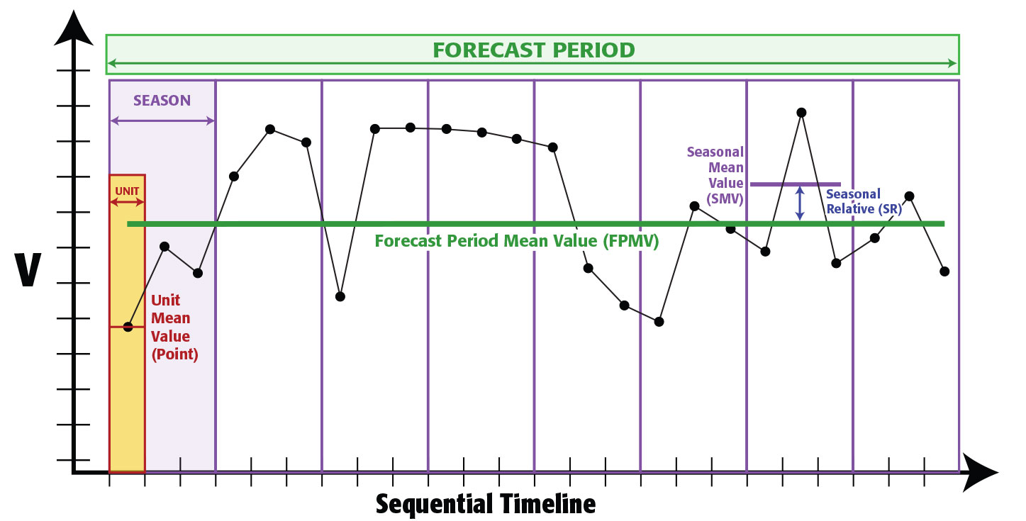
Figure 1: Units, Seasons, and Periods of Time
The forecast period for the current library of seasonal models is a calendar month. This is the defining container used to compute the seasonal relatives for each individual season. The SMV of each season is the mean of each unit value of each season within the calendar month. The FPMV is the mean value of each unit value of the entire calendar month.
Each forecast value is the product of the base forecast and the Forecasted Seasonal Relative (FSR) of that season. The FSR is the result of a simple moving average of the most recent historical SR values of the season.
Each seasonal model is expressed as a matrix. Each instance of each season has a unique identifier, and this identifier is how each current season is linked with the previous instances of that season along the seasonal timeline.
Let’s consider how this works with the Week Day seasonal model. The Week Day seasonal model is calendar-based. It consists of seven seasons: the seven days of the week.
The Week Day seasonal model is non-contiguous. Each season includes either four or five non-contiguous values within each calendar month. The SMV of “Monday” is the average of the daily value of each Monday in that calendar month.
Each specific seasonal instance is designated as [Season]-[Year]-[Quarter]-[Month]. For example, Mon-2024-Q1-Feb, or Thu-2022-Q3-Sep. These unique season identifiers facilitate linking the historical instances of each season across three different series designated s (season), sq (season-quarter), and sqm (season-quarter-month).
The historical cycles of the “s” series take the three most recent instances of the season. If the current season is Fri-2026-Q1-Feb, p1_msr would be Fri-2026-Q1-Jan, p2_msr would be Fri-2025-Q4-Dec, and p3_msr would be Fri-2025-Q4-Nov.
The historical cycles of the “sq” series take the three most recent instances of the season in the same quarter. So if the current season is Fri-2026-Q1-Feb, p1_msr would be Fri-2026-Q1-Jan, p2_msr would be Fri-2025-Q1-Mar, and p3_msr would be Fri-2025-Q1-Feb.
The historical cycles of the “sqm” series take the three most recent instances of the season in the same quarter and the same month. If the current season is Fri-2026-Q1-Feb, p1_msr would be Fri-2025-Q1-Feb, p2_msr would be Fri-2024-Q1-Feb, and p3_msr would be Fri-2023-Q1-Feb.
Each of these lenses uses the same seasonal model, but each reveals different historical patterns. Moreover, the amount of historical data becomes a critical factor when selecting which lens to use. The wd-s series has 12 historical instances of each season each calendar year. With 2 years of historical data, every season has at least 24 accuracy metrics, which is statistically significant without becoming unwieldy. Forecasts with the wd-sq series would each have 6 historical instances with 2 years of historical data, which still clear the minimum requirement of 5 historical instances. But forecasts with the wd-sqm series would each have only 2 historical instances with 2 years of historical data.
With 20 years of historical data, forecasts with the wd-s series would each have 240 historical examples and the forecasted margin of error would be the mean of 240 historical errors. Forecasts with the wd-sq series would each have 60 historical instances, and forecasts with the wd-sqm would each have 20 historical instances.
A Universe of Seasonal Models
Developing new seasonal models that aren’t based on the calendar is more challenging than you might think. Time is circular and cyclical. To measure time we require some kind of external, objective reference to mark the start of each cycle. Even the calendar and the clock require an external, objective reference. The external, objective references human beings use to measure time are celestial.
The calendar and the clock are based on the observed cycles of the Sun as it appears to orbit the Earth. While days and years are based on the observed cycles of the Sun, the concept of a month is based on the observed cycles of the Moon. We measure and understand time in terms of the calendar and the clock, and we take these systems for granted without considering how and why they were established.
The calendar exists so that farmers can accurately predict the changes of the seasons. The reason for the complicated system of Leap Years in the Gregorian Calendar is so that the Spring Equinox—an external, observable, celestial event—always falls between March 20th and March 21st.
Standardized clock times and time zones exist so that trains can run on time. Until November 18, 1883, when North America adopted “Railroad Time,” which divided the continent into four time zones, each set one hour apart, all time in the United States was local and the country had over 300 individual time zones. And you were today years old when you learned that the branch of the government in charge of time zones and Daylight Savings is the U.S. Department of Transportation.
The calendar-based seasonal models, including the Calendar Month, Week Year, Week Day, and Month Day models, are based on the observed cycles of the Sun. They’re examples of regular seasonality.
Regular seasonality is regular because the duration of the individual seasons of a seasonal model is uniform, the sequence of seasons is consistent, and the cycles of the season fit within the larger container of a calendar year, so that each season occurs at least once during each calendar year.
Seasonal models based on the observed cycles of planets other than the Sun are examples of irregular seasonality. Irregular seasonality is irregular because the duration of the individual seasons of a seasonal model can vary from instance to instance, the sequence of the seasons is inconsistent and variable, and the cycles of the season do not fit within the larger container of a calendar year, so not every season occurs every year.
The other 78 seasonal models in the TSF Inc. library are complex, irregular seasonal models based on the observed cycles of the Moon, Mercury, and Venus. These lenses include models with as many as 204 and as few as 3 seasons. The average duration of individual seasons ranges from 1 to 30 days with most seasons consisting of from 4 to 15 contiguous calendar days.
The forecasts on the TSFStocks.com website consider 30 different seasonal models, selected to provide the optimal coverage for historical data from 5 to 30 years.