
What separates success from failure — in every business, in every market — is timing. Every business owner, every operator, every financial manager knows WHAT to do. They just don’t know WHEN to do it. The cost of getting the timing wrong is catastrophic. A retailer who reorders late loses the sale. A restaurant that overpreps eats the margin. A manufacturer who ramps early bleeds cash. A fund manager who buys at the wrong time loses the fund. Solving the timing problem is the sole purpose of forecasting.
The entire discipline of time series forecasting exists to answer one question: “WHAT will the next number be?” The spectrum of forecast models from simple moving averages to complex machine learning and multi-variable neural network configurations represents variations on HOW to answer that question. The problem isn’t merely that this is the wrong question: you don’t need to know WHAT the next number will be; you need to know WHEN to act. The problem is that this question is impossible to answer with any degree of certainty.
The theory of time series forecasting is sound: structural patterns in the past tend to continue in the future. The problem is finding those structural patterns in the first place. Legacy forecasting models look for internal (endogenous) structural patterns — patterns in the data itself. This is why legacy forecasting models are doomed to fail. They ask the wrong question, and they look for structural patterns in the wrong place.
AI Is an Extraordinarily Powerful Tool Solving the Wrong Problem
To appreciate why AI can’t solve the timing problem, we first need to understand why and how AI is being applied to the discipline of time series forecasting. The premise of time series forecasting is that learnable patterns exist in historical time series data, and those patterns predict future values. For more than 50 years this approach has failed consistently. No matter what patterns humans identify in the historical data, those patterns fail to predict the future with any level of statistical significance. The most sophisticated forecast models look for patterns by considering correlations among the historical data, and this is the role that AI performs. Every application of AI is intended to find patterns in the historical data that human intelligence can’t find.
The problem is that the patterns AI is looking for don’t exist in the data.
AI identifies correlation among the data — but correlation is descriptive, not predictive. Correlation describes a relationship among the data but it doesn’t identify what causes that relationship. This isn’t a limitation of AI: it’s the fatal flaw in every legacy forecasting model.
Legacy Time Series Forecasting Confuses Correlation with Causation
Every legacy time series forecasting model asks the question, “What will the next number be.” This question assumes that each value in a time series causes the next. Every mathematical formula used in time series forecasting assumes that each value is the effect of the previous value. This is a fatally flawed assumption. Today’s stock price doesn’t make tomorrow’s stock price happen. Yesterday’s demand didn’t make today’s demand happen. Time series forecasting models correlation, not causation. Each value in a time series is the effect of external (exogenous) forces at different points in time. The correlations among the values exist because the external conditions persist, not because the values influence each other.
In other words, the structural patterns that make time series forecasting possible are external not internal. Every failure of legacy forecasting is the consequence of looking for internal structure in the data. These are not mere mistakes that can be corrected or overcome with AI. Legacy forecasting models are built on the assumption of internal structure. Legacy forecasting models assume a single causal chain — each value determined by the values that precede it — and are therefore incapable of considering external structure. The failures of legacy forecasting are systemic and inevitable because the process is subjective.
The Process Is Subjective Because it Lacks Structure
Structure is the prerequisite for objectivity. Structure defines where to start, where to stop, what to measure, and how to evaluate. Without structure, every decision in the forecasting process is a judgment call. Every judgment call is defensible, and therein lies the true problem. A subjective process lacks a single source of truth, and without a single source of truth, it’s not possible to know WHEN to act.
The Search for Patterns Is Recursive and Endless
Because legacy forecasting models lack external, objective references, they look for patterns by segmenting the historical data into a training segment and a testing segment. They look for correlations among the data in the training segment, and then test those correlations in the testing segment, adjusting for errors, fitting curves, and cycling between training and testing until the pattern in the training data is reflected in the testing data. The assumption of this process is that correcting for past errors will make future forecasts more accurate — and yet practitioners know that assumption is unsupported.
Rather than accepting that the entire process is futile, practitioners assume that success is a matter of balance. Failures with this approach are blamed on “overfitting” where the testing data is so perfectly aligned to the training data that it’s incapable of adapting to new data. But without external, objective references, it’s impossible to know when to stop tuning the model.
The problem is that sometimes, objective patterns exist in the data. The only instance where legacy forecasting models consider the dimension of time is when looking for “seasonality.” In some sets of data, clear patterns of peaks and troughs exist along the sequential timeline. The textbook example is the data of fatal highway car crashes, where the most fatalities occur on Saturdays, and the fewest occur on Tuesdays. Not only is this pattern objective, it can also be seen with the naked eye. “Seasonality” is the sole objective internal pattern in time series data, and yet rather than embracing it, legacy forecasting models intentionally strip it out of historical data because it makes finding subjective patterns more difficult.
Every Backtest Fails When Faced With New Data
Legacy forecasting models “train” on historical data to settle on the specific parameters of the proposed forecast signal. The results are presented as a backtest: an example of how well the selected forecast model — which was trained and tested on the historical data — is able to forecast that same historical data. The assumption is that because the model performed so well with the historical data, it will continue to perform well with new data. This is never true.
Every backtest fails when faced with new data. But the problem is bigger than this. The entire industry presents backtests as evidence, and yet no one trusts backtests. Backtests are performative. All that matters is how well the model works with new, out-of-sample data. Even if the model performs well initially, it will fail inevitably. The model will be abandoned, and the subjective search for patterns will begin again.
Every Forecast Model Is Equal
The lack of objectivity means that every forecast model fails equally on out-of-sample data. It doesn’t matter how well a model predicted the past. The most advanced AI-powered forecast model can’t predict the next number any better than a simple moving average can.
This is not conjecture. The M-Competition, the most comprehensive empirical evaluation of forecasting methods ever conducted, found that simple methods match or outperform complex models on out-of-sample data. More computation, more parameters, and more sophistication produce no improvement. Forecast models are broken clocks: they’re right twice a day, but none of the current tools can tell you WHEN a given model will be right.
The End of the Timing Problem
The biggest irony — and the ultimate source of these failures — is that the current discipline of time series forecasting doesn’t actually consider the dimension of time. Legacy forecasting models claim to address time because they ask what the NEXT number will be, but NEXT relates to sequence, not to time. Knowing WHAT the next number will be doesn’t tell you WHEN to act.
Legacy forecasting models are incapable of solving the timing problem because legacy forecasting models do not consider time. TSF solves the timing problem because TSF is the science of WHEN.
Temporal Structural Forecasting: The Science of WHEN
The timing problem persists because it’s complex. Legacy forecasting tools fail to solve the timing problem because they’re simple. They’re necessary to solve the timing problem, but they’re not sufficient. Legacy forecasting tools are designed to predict WHAT the next number will be, not WHEN conditions have changed. They can’t address the timing problem because they don’t consider the dimension of time. Legacy forecasting tools require objective structure to forecast the number, but they can only look for that structure internally, within the data. These limitations are two sides of the same coin: the structure legacy forecast models require exists in the dimension of time.
What legacy forecasting models call “seasonality” in time series data is in fact evidence that temporal structure exists. The observed pattern in the data is the effect of temporal structure on the independent values in the time series. Seasonality isn’t the only temporal structure that exists; it’s merely the only type of temporal structure that can be seen with the naked eye.
TSF Inc. has invented a Microscope for Time, the result of more than 7 years of independent research into the dimension of time itself. When time series data is viewed through the “lenses” of complex, irregular seasonal models, we can see objective structural patterns that are not only invisible to the naked eye, but also undetectable with AI.
The Microscope for Time identifies the missing structure required by legacy forecasting models, but it doesn’t allow legacy forecasting models to consider the dimension of time. Legacy forecasting models consider a single axis, the sequential timeline. This is sufficient to define WHAT the number will be, but not WHEN it will change. The Temporal Structural Forecasting methodology can address both WHAT and WHEN because it forecasts along two timelines, the sequential timeline and the seasonal timeline, using the Model of Temporal Inertia.
The Model of Temporal Inertia: How Time Series Forecasting Works
Newton’s First Law of Motion, the Law of Inertia states that an object at rest remains at rest and an object in motion remains in motion in constant speed and in a straight line unless acted on by an unbalanced force. The Model of Temporal Inertia proposes that the values of data organized in a time series will follow the same trend (speed and direction) until acted on by an unbalanced force.
Legacy forecasting models require stationary data, and go so far as to decompose the time series data to remove every possible external influence, including trend, seasonality, and random noise. Effectively, legacy forecasting models filter out the effect of the unbalanced forces at different points in time to forecast the inertial trend — the mean value that will remain constant across the entire forecast horizon until acted on by an unbalanced force.
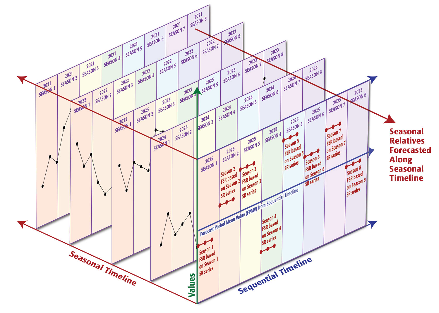
The Model of Temporal Inertia proposes that the relative effect of these unbalanced forces at each point in time can be quantified and expressed as a seasonal relative. Each historical value in the time series can be expressed as the product of the inertial trend and the seasonal relative. Each future value in the time series can be expressed as the product of the forecast period mean value —the legacy forecast value—and the forecasted seasonal relative.
The complex, irregular seasonal models that comprise the Microscope for Time define objective boundaries of each season, which are used to calculate the seasonal relative value for each instance of each season. The next seasonal relative value in the sequence is forecast along the seasonal timeline, and then combined with the value of the inertial trend, forecast along the sequential timeline.
The sequential timeline is the familiar ordered linear progression of time. On the sequential timeline, Season 6 of 2026 follows Season 5 of 2026, which follows Season 4 of 2026. The seasonal timeline is perpendicular to the sequential timeline. On the seasonal timeline, Season 6 of 2026 follows Season 6 of 2025, which follows Season 6 of 2024.
Legacy forecasting models time series data on two axes: the sequential timeline and the value. Temporal Structural Forecasting, based on the Model of Temporal Inertia, models time series data with three axes: the sequential timeline, the seasonal timeline, and the value. This overcomes every limitation and failure inherent in legacy forecasting models.
Patterns Are Objective and External
Legacy forecasting models identify the inertial trend of the data along the sequential timeline. Temporal Structural Forecasting (TSF) uses the Microscope for Time to quantify the relative effects of the external unbalanced forces at each point in time. The “lenses” in the Microscope for Time are matrices that map each calendar date to a specific season in the seasonal model. The mean of the historical values of each calendar date contained within a season is used to calculate the seasonal relative of that season. The historical seasonal relatives of each season form a time series along the seasonal timeline, and the next value in this series is the forecasted seasonal relative: the expected effect of the external unbalanced forces during the next instance of the season.
Each forecast value is the product of two single-period forecasts on two independent timelines. The base forecast value is the forecasted inertial trend: the expected mean value for the entirety of the weekly, monthly, or quarterly forecast period. The forecasted seasonal relatives use the seasonal timeline to model how the variable effects of the external unbalanced forces affect the forecasted inertial trend.
This is why TSF can forecast an entire month of daily values at once, with no loss of confidence. When forecasting on a single timeline, each value is dependent on the previous forecast value, and the errors increase exponentially. When forecasting on two timelines, each forecast value is independent, and the forecast errors do not compound.
Objective Historical Analysis Succeeds Where Subjective Backtests Fail
Until now, any evidence of historical performance was a subjective backtest, and therefore inherently performative and unreliable. Because backtests are the only way to consider historical performance of legacy forecast models, and legacy forecast models have been the only available options, everyone assumes that all historical analysis is a subjective, performative backtest that cannot be trusted. Historical analysis of TSF forecasts does not use backtests.
Backtests fail because they are inherently subjective and recursive. They are examples of how well the selected forecast model — which was trained and tested on the historical data — is able to forecast that same historical data. Temporal Structural Forecasting involves no training, testing, or tuning of the forecasts. Every historical forecast is out-of-sample because no part of the historical data is used for in-sample training.
The methodology used for the financial forecasts is designed to make leakage impossible. The forecast is generated entirely from historical closing prices. No intraday price — no open, no high, no low — enters the forecast computation. The forecasted BUY signals, the daily values of the lower confidence band are generated one week in advance, so the forecast exists before the outcome. The trade executes entirely on intraday prices. Entry triggers when the stock’s intraday low touches the confidence band — a price computed from the closing prices and delivered before the trading week began. Exit triggers when the intraday high reaches the 5% profit target, or the position closes after 120 days. The forecast and the trade share no data. They are connected only by the limit order price: a one-way gate from the forecast to the trade, never in the reverse direction.
Because TSF timing signals use objective, external temporal structure, how well they performed in the past is a reliable indicator of how well they will perform in the future. More importantly, research has shown that the TSF timing signals have maintained or recovered structural integrity across 14 major market shocks including Bear Stearns and Lehman, the U.S. Debt Downgrade, Brexit, Volmageddon, and COVID-19.
Every Equal Forecast Model Competes for Confidence
Every forecast model fails equally. Forecast models are broken clocks: they’re right twice a day. But the TSF methodology compares the historical patterns of accuracy of multiple forecast models across individual seasons along the seasonal timeline to determine WHEN a given model can be trusted.
Each combination of a seasonal model, a base forecast, and a forecasted seasonal relative constitutes a single unique forecast model. Currently, TSF Inc. has a library of 81 seasonal models, a choice of 8 base forecasts, and 6 different seasonal relative options, or a population of 3,888 unique, objective forecast models. In practice, TSF considers from 30 to 800 forecast models at a time. Each forecast value is produced using each forecast model. The historical patterns of accuracy of each forecast model for each date are then ranked, and the forecast model with the best historical pattern of accuracy for that date is selected. The process is 100% objective and requires no human intervention or judgment calls.
The TSF methodology uses those historical patterns of accuracy to assign objective confidence bands to each forecast value, identifying the range where actual values should land under normal conditions. If the actual values fall outside of this range, it’s not an error in the forecast, it’s a signal that conditions right now are not normal.
The “map of normal” is how TSF tells you WHEN to act.